Automating data loading from multiple files
In this example, we will show how to load into Tengri data that is stored as multiple .parquet files in the storage of S3.
Using the Python boto3 module, we will output the paths of all .parquet files in a particular storage:
import boto3
import boto3.s3.transfer

path = 'Stage/<lake_path>/DataLake/2049/'
s3_client = boto3.client('s3',
                        endpoint_url='***',
                        aws_access_key_id='***',
                        aws_secret_access_key='***',
                        region_name='us-east-1')

response = s3_client.list_buckets()

for bucket in response['Buckets']:
    print(f'Bucket: {bucket["Name"]}')
    response = s3_client.list_objects_v2(
    Bucket=bucket["Name"],
    Prefix='Stage')

    for content in response.get('Contents', []):
        file_path = str(content['Key'])
        if path in file_path:
            print(file_path)
Bucket: prostore
Stage/<lake_path>/DataLake/2049/1.parquet
Stage/<lake_path>/DataLake/2049/2.parquet
Stage/<lake_path>/DataLake/2049/3.parquet
Stage/<lake_path>/DataLake/2049/4.parquet
Stage/<lake_path>/DataLake/2049/5.parquet
Bucket: s3bench-asusnode21Let’s try querying SQL for data from one of these files and make sure that the query is processed and the data is displayed in the output:
SELECT *
    FROM read_parquet('s3://prostore/Stage/<lake_path>/DataLake/2049/1.parquet')
LIMIT 5;
+-----------------------------------------------------------------------------------------------------------------------------+-------+---------------------+----------------------------+----------+----------+----------------------------+-------------------------+
| f1 | f2 | f3 | f4 | jd1 | jd2 | command_load_datetime | command_load_session_id |
+-----------------------------------------------------------------------------------------------------------------------------+-------+---------------------+----------------------------+----------+----------+----------------------------+-------------------------+
| {"id": 673, "age": 77, "name": "d1b7d724ef3a8451189fc47da62b9888", "email": "b32c9c5d3b1768e7955144103d72c593@example.com"} | false | 0001-01-02 06:44:06 | <memory at 0x7f0bb8523880> | 7000-1-1 | 7000-2-1 | 2025-06-23 08:05:23.636063 | 195 |
+-----------------------------------------------------------------------------------------------------------------------------+-------+---------------------+----------------------------+----------+----------+----------------------------+-------------------------+
| {"id": 221, "age": 34, "name": "4de35c863a2df55018eca39f130c0738", "email": "3535ac8c3b04c33ac67ee70693707bdb@example.com"} | true | 0001-01-02 02:59:53 | <memory at 0x7f0bb85219c0> | 7000-1-1 | 7000-2-1 | 2025-06-23 08:05:23.636063 | 195 |
+-----------------------------------------------------------------------------------------------------------------------------+-------+---------------------+----------------------------+----------+----------+----------------------------+-------------------------+
| {"id": 612, "age": 27, "name": "94a027942dffccb4abe3923914592ba5", "email": "10178786f4378e98f62be257c4215056@example.com"} | false | 0001-01-02 11:53:53 | <memory at 0x7f0bb8522c80> | 7000-1-1 | 7000-2-1 | 2025-06-23 08:05:23.636063 | 195 |
+-----------------------------------------------------------------------------------------------------------------------------+-------+---------------------+----------------------------+----------+----------+----------------------------+-------------------------+
| {"id": 136, "age": 73, "name": "500522adeb682c1efcdce8af83610a27", "email": "de507ff06310d2b35ea65c40f26f6a94@example.com"} | false | 0001-01-02 00:56:43 | <memory at 0x7f0bb8521fc0> | 7000-1-1 | 7000-2-1 | 2025-06-23 08:05:23.636063 | 195 |
+-----------------------------------------------------------------------------------------------------------------------------+-------+---------------------+----------------------------+----------+----------+----------------------------+-------------------------+
| {"id": 150, "age": 67, "name": "7d283d7c78b5692f6162d8b65baee1ed", "email": "df78cebca3c40d06e8b43ad8a7e98f56@example.com"} | true | 0001-01-02 13:46:41 | <memory at 0x7f0bb8521600> | 7000-1-1 | 7000-2-1 | 2025-06-23 08:05:23.636063 | 195 |
+-----------------------------------------------------------------------------------------------------------------------------+-------+---------------------+----------------------------+----------+----------+----------------------------+-------------------------+Now we need to load the data from all the .parquet files into one table.
To do this, first initialise this table — create it, but do not write data to it yet, so that we can do it in the next step with a loop.
To initialise the table, execute this command with the SELECT * subquery for one of these files and the LIMIT — 0 parameter:
CREATE OR REPLACE TABLE raw_dyntest AS
    SELECT *
        FROM read_parquet('s3://prostore/Stage/<lake_path>/DataLake/2049/1.parquet')
    LIMIT 0;
Done in 22.2 sec
+--------+
| status |
+--------+
| CREATE |
+--------+This query creates a table with the required set of columns and their types, now we can load data into it in a loop.
For this purpose, in the cell of type Python we will describe a loop by the names of all files and in this loop using the function tngri.sql we will iteratively load data from each file .parquet into the initialised table raw_dyntest.
In each iteration we will output the number of rows in this table that should increment.
import tngri

for i in range(1,6):
    file_name = f"s3://prostore/Stage/<lake_path>/DataLake/2049/{i}.parquet"
    insert_sql = f"INSERT INTO raw_dyntest SELECT * FROM read_parquet('{file_name}')"
    print(insert_sql)
    tngri.sql(insert_sql)

    print(tngri.sql("SELECT count(*) FROM raw_dyntest"))
insert into raw_dyntest select * from read_parquet('s3://prostore/Stage/<lake_path>/DataLake/2049/1.parquet')
shape: (1, 1)
+----------+
│ column_0 │
│ --- │
│ i64 │
+----------+
│ 10000000 │
+----------+
insert into raw_dyntest select * from read_parquet('s3://prostore/Stage/<lake_path>/DataLake/2049/2.parquet')
shape: (1, 1)
+----------+
│ column_0 │
│ --- │
│ i64 │
+----------+
│ 20000000 │
+----------+
insert into raw_dyntest select * from read_parquet('s3://prostore/Stage/<lake_path>/DataLake/2049/3.parquet')
shape: (1, 1)
+----------+
│ column_0 │
│ --- │
│ i64 │
+----------+
│ 30000000 │
+----------+
insert into raw_dyntest select * from read_parquet('s3://prostore/Stage/<lake_path>/DataLake/2049/4.parquet')
shape: (1, 1)
+----------+
│ column_0 │
│ --- │
│ i64 │
+----------+
│ 40000000 │
+----------+
insert into raw_dyntest select * from read_parquet('s3://prostore/Stage/<lake_path>/DataLake/2049/5.parquet')
shape: (1, 1)
+----------+
│ column_0 │
│ --- │
│ i64 │
+----------+
│ 50000000 │
+----------+Now let’s display the number of rows in the table filled in this way:
SELECT count(*) AS row_count
    FROM raw_dyntest;
+-----------+
| row_count |
+-----------+
| 50000000 |
+-----------+To check that queries to this data on such a volume (50 million rows) work properly, let’s display the distribution of true and false values in the f2 column:
SELECT f2, count(*) AS f2_cnt
    FROM raw_dyntest_ng
    GROUP BY f2;
+-------+----------+
| f2 | f2_cnt |
+-------+----------+
| false | 24998577 |
+-------+----------+
| true | 25001423 |
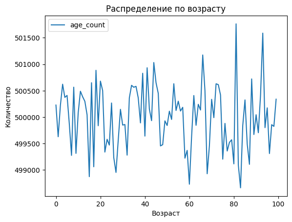
+-------+----------+One of the columns of the table contains data in the form of JSON structure, and one of the keys of this structure is age. Let’s build a table of age values distribution. To do this, use the function json_extract.
SELECT
    json_extract(f1, ['age'])[1]::INT AS age,
    count(*) AS age_count
    FROM raw_dyntest
    GROUP BY 1 ORDER BY 1;
Done in 9.9 sec
+-----+-----------+
| age | age_count |
+-----+-----------+
| 0 | 500228 |
+-----+-----------+
| 1 | 499629 |
+-----+-----------+
| 2 | 500222 |
+-----+-----------+
| 3 | 500622 |
+-----+-----------+
| 4 | 500373 |
+-----+-----------+
| 5 | 500410 |
+-----+-----------+
| 6 | 499876 |
+-----+-----------+
| 7 | 499276 |
+-----+-----------+
| 8 | 500566 |
+-----+-----------+
| 9 | 499314 |
+-----+-----------+
| ... | ... |
+-----+-----------+Based on this table, plot the distribution of values by age:
import matplotlib

plt = cell_output.plot(
    title='Распределение по возрасту',
    y='age_count',
    ylabel='Количество',
    x='age',
    xlabel='Возраст',
)

plt.get_figure()